#04 | Overfitting & Hyperparameter Tuning with Cross Validation

Chapter Importance

We have already covered:

1. Regression Models

2. Classification Models

3. Train Test Split for Model Selection

In short, we have computed all possible types of models to predict numerical and categorical variables with Regression and Classification models, respectively.

Although it is not enough to compute one model, we need to compare different models to choose the one whose predictions are the closest to reality.

Nevertheless, we cannot evaluate the model on the same data we used to .fit() (train) the mathematical equation (model). Therefore, we need to separate the data into train and test sets; the first to train the model, the later to evaluate the model.

We add an extra layer of complexity because we can improve a model (an algorithm) by configuring its parameters. This chapter is about computing different combinations of a single model's hyperparameters to get the best.

Load the Data

• The goal of this dataset is

• To predict if bank's customers (rows) default next month

• Based on their socio-demographical characteristics (columns)

import pandas as pd
pd.set_option("display.max_columns", None)

url = 'https://archive.ics.uci.edu/ml/machine-learning-databases/00350/default%20of%20credit%20card%20clients.xls'
df_credit = pd.read_excel(io=url, header=1, index_col=0)
df_credit.sample(10)

Preprocess the Data

Missing Data

The function .fit() needs all the cells in the DataFrame to contain a value. NaN means "Not a Number" (i.e., cell for which we don't have any information). Otherwise, it won't know how to process the row and compare it to others.

df_credit.isna().sum()

LIMIT_BAL 0 SEX 0 .. PAY_AMT6 0 default payment next month 0 Length: 24, dtype: int64

df_credit.isna().sum().sum()

0

Dummy Variables

The function .fit() needs the values to be numeric. Otherwise, Python won't know the position of the axes in which to allocate the point.

Therefore, categories of the categorical columns will be transformed into new columns (one new column per category) and contain 1s and 0s depending on whether the person is or is not in the category.

Nevertheless, we don't need to create dummy variables because the data contains numerical variables only.

Feature Selection

So far, we have used the naming standard of target and features. Nevertheless, the most common standards on the Internet are X and y. Let's get used to it:

y = df_credit.iloc[:, -1]
X = df_credit.iloc[:, :-1]

Train Test Split

From the previous chapter, we should already know we need to separate the data into train and test if we want to evaluate the model's predictive capability for data we don't know yet.

In our case, we'd like to predict if new credit card customers won't commit default in the next month. As we don't have the data for the next month (it's the future), we need to apply the function train_test_split().

from sklearn.model_selection import train_test_split

X_train, X_test, y_train, y_test = train_test_split(
    X, y, test_size=0.33, random_state=42)

DecisionTreeClassifier() with Default Hyperparameters

To compute a Machine Learning model with the default hyperparameters, we apply the same procedure we have covered in previous chapters:

from sklearn.tree import DecisionTreeClassifier

model_dt = DecisionTreeClassifier()
model_dt.fit(X_train, y_train)

DecisionTreeClassifier()

Accuracy

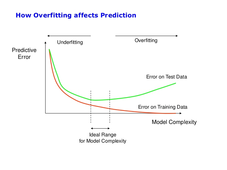
We can see the model is almost perfect for predicting the training data (99% of accuracy). Nevertheless, predicting test data is terrible (72% of accuracy). This phenomenon tells us that the model is incurring in overfitting.

In train data

model_dt.score(X_train, y_train)

0.9995024875621891

In test data

model_dt.score(X_test, y_test)

0.7265656565656565

Model Visualization

I'll use the following visualization to explain the concept of overfitting.

from sklearn.tree import plot_tree

plot_tree(decision_tree=model_dt, feature_names=X_train.columns, filled=True);

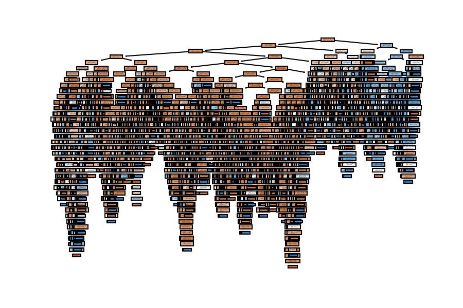
The tree is big because we have a lot of people (20,100), and we haven't set any limit on the model.

How many people do you think we have in the deepest leaf?

• Very few, probably one.

Are these people characteristic of the overall data? Or are they infrequent?

• Because they are infrequent and the model is very complex, we are incurring overfitting, and we get a vast difference between train and test accuracies.

DecisionTreeClassifier() with Custom Hyperparameters

Which hyperparameters can we configure for the Decision Tree algorithm?

In the output below, we can configure parameters such as max_depth, criterion and min_samples_leaf, among others.

model = DecisionTreeClassifier()

model.get_params()

{'ccp_alpha': 0.0, 'class_weight': None, 'criterion': 'gini', 'max_depth': None, 'max_features': None, 'max_leaf_nodes': None, 'min_impurity_decrease': 0.0, 'min_samples_leaf': 1, 'min_samples_split': 2, 'min_weight_fraction_leaf': 0.0, 'random_state': None, 'splitter': 'best'}

Let's apply different random configurations to see how to model's accuracy changes in train and test sets.

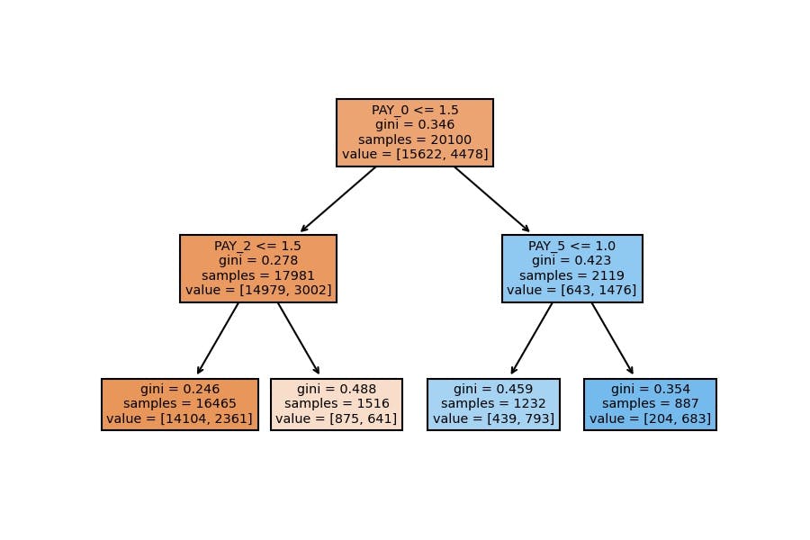
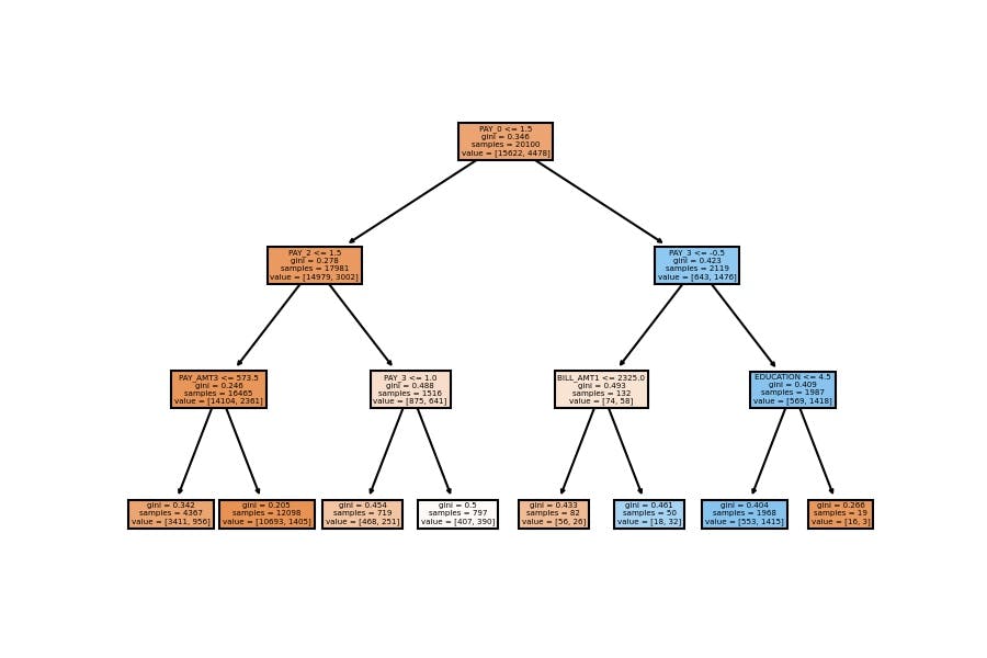
Please pay attention to how the accuracies are similar when we reduce the model's complexity (we make the tree shorter and generalized to capture more people in the leaves).

And remember that we should pick up a good configuration based on the test accuracy.

1st Configuration

model_dt = DecisionTreeClassifier(max_depth=2, min_samples_leaf=150)
model_dt.fit(X_train, y_train)

DecisionTreeClassifier(max_depth=2, min_samples_leaf=150)

Accuracy

In train data

model_dt.score(X_train, y_train)

0.8186567164179105

In test data

model_dt.score(X_test, y_test)

0.8215151515151515

Model Visualization

plot_tree(decision_tree=model_dt, feature_names=X_train.columns, filled=True);

Learn how to become an independent Machine Learning programmer who knows when to apply any ML algorithm to any dataset.

2nd Configuration

model_dt = DecisionTreeClassifier(max_depth=3)
model_dt.fit(X_train, y_train)

DecisionTreeClassifier(max_depth=3)

Accuracy

In train data

model_dt.score(X_train, y_train)

0.8207960199004976

In test data

model_dt.score(X_test, y_test)

0.8222222222222222

Model Visualization

plot_tree(decision_tree=model_dt, feature_names=X_train.columns, filled=True);

3rd Configuration

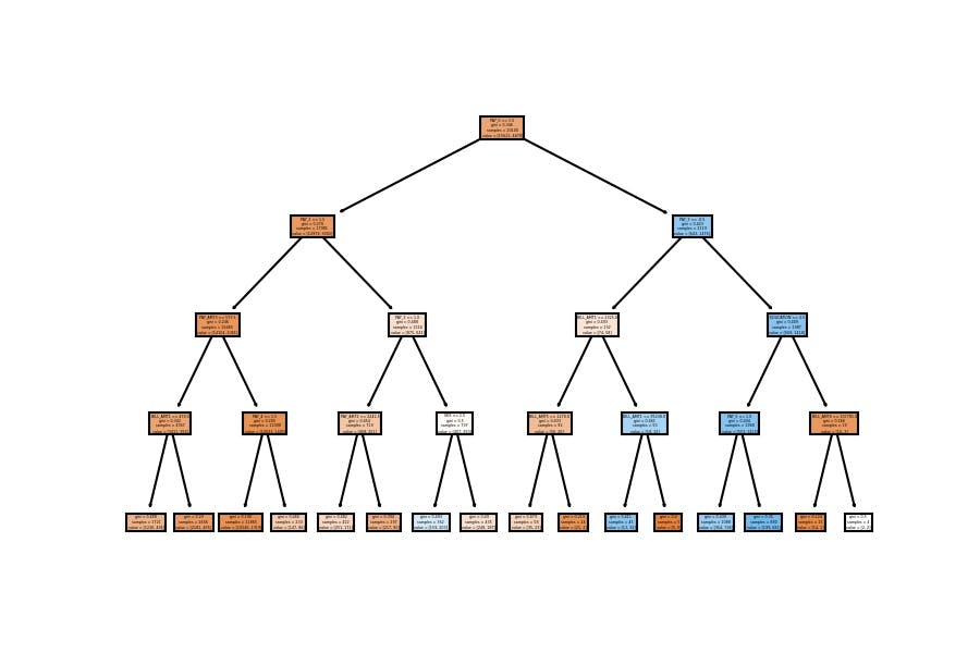
model_dt = DecisionTreeClassifier(max_depth=4)
model_dt.fit(X_train, y_train)

DecisionTreeClassifier(max_depth=4)

Accuracy

In train data

model_dt.score(X_train, y_train)

0.8232338308457712

In test data

model_dt.score(X_test, y_test)

0.8205050505050505

Model Visualization

plot_tree(decision_tree=model_dt, feature_names=X_train.columns, filled=True);

4th Configuration

Accuracy

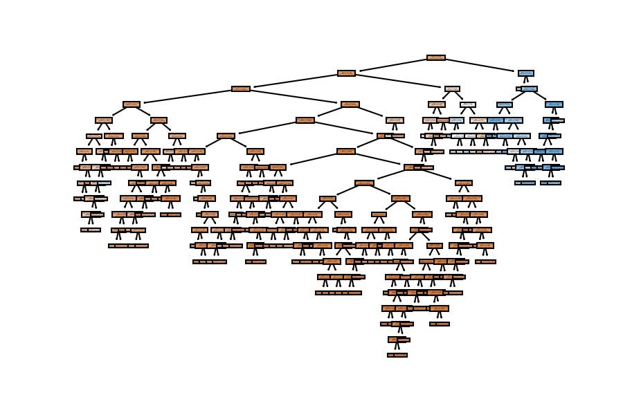
model_dt = DecisionTreeClassifier(min_samples_leaf=100)
model_dt.fit(X_train, y_train)

DecisionTreeClassifier(min_samples_leaf=100)

In train data

model_dt.score(X_train, y_train)

0.8244278606965174

In test data

model_dt.score(X_test, y_test)

0.8161616161616162

Model Visualization

plot_tree(decision_tree=model_dt, feature_names=X_train.columns, filled=True);

5th Configuration

model_dt = DecisionTreeClassifier(max_depth=7, min_samples_leaf=100)
model_dt.fit(X_train, y_train)

DecisionTreeClassifier(max_depth=7, min_samples_leaf=100)

Accuracy

In train data

model_dt.score(X_train, y_train)

0.8237313432835821

In test data

model_dt.score(X_test, y_test)

0.8177777777777778

Model Visualization

plot_tree(decision_tree=model_dt, feature_names=X_train.columns, filled=True);

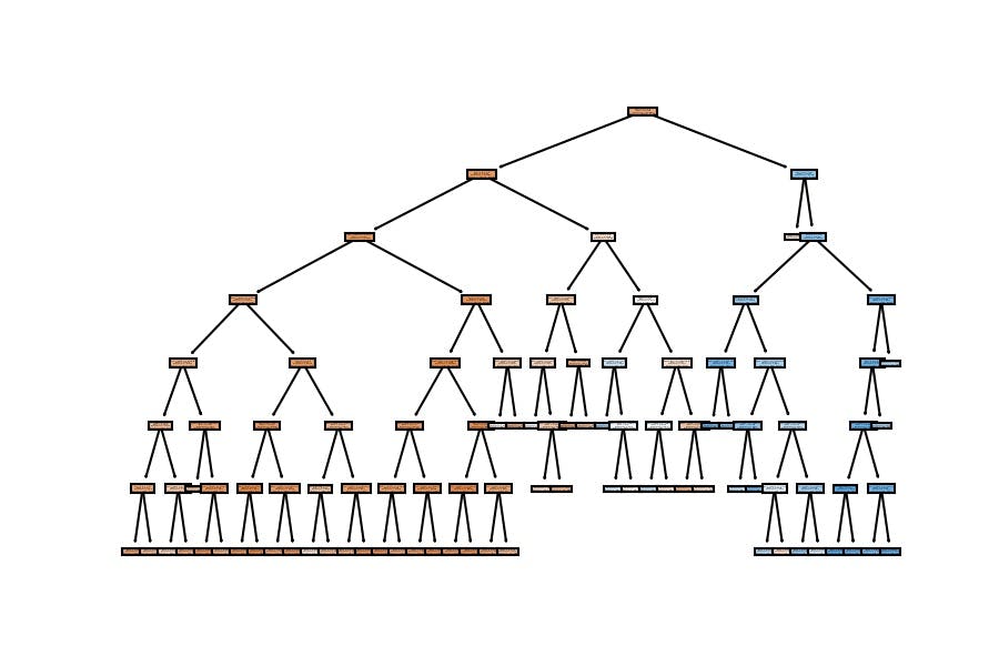
We have similar results; the accuracy goes around 82% on the test set when we configure a general model which doesn't have a considerable depth (as the first one).

But we should ask ourselves another question: can we do this process of automatically checking multiple combinations of hyperparameters?

• Yes, and that's where Cross Validation gets in.

GridSearchCV() to find Best Hyperparameters

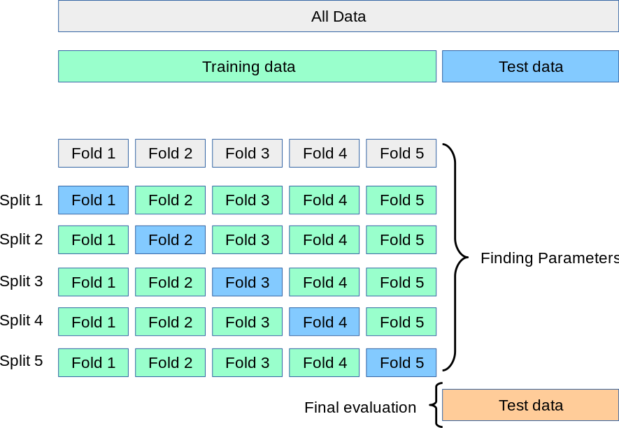
The Cross-Validation technique splits the training data into n number of folds (5 in the image below). Then, it computes each hyperparameter configuration n times, where each fold will be taken as a test set once.

Consider that we .fit() a model as many times as folds are multiplied by the number of combinations we want to try.

Out of the Decision Tree hyperparameters:

model_dt = DecisionTreeClassifier()

model_dt.get_params()

{'ccp_alpha': 0.0, 'class_weight': None, 'criterion': 'gini', 'max_depth': None, 'max_features': None, 'max_leaf_nodes': None, 'min_impurity_decrease': 0.0, 'min_samples_leaf': 1, 'min_samples_split': 2, 'min_weight_fraction_leaf': 0.0, 'random_state': None, 'splitter': 'best'}

We want to try the following combinations of max_depth (6), min_samples_leaf (7) and criterion (2):

from sklearn.model_selection import GridSearchCV

param_grid = {
    'max_depth': [None, 2, 3, 4, 5, 10],
    'min_samples_leaf': [1, 50, 100, 200, 400, 800, 1600],
    'criterion': ['gini', 'entropy']
}

cv_dt = GridSearchCV(estimator=model_dt, param_grid=param_grid, cv=5, verbose=1)

They make up to 420 times we compute the function.fit()

5*6*7*2

420

To compare 84 different combinations of the Decision Tree hyperparameters:

6*7*2

84

cv_dt.fit(X_train, y_train)

Fitting 5 folds for each of 84 candidates, totalling 420 fits

GridSearchCV(cv=5, estimator=DecisionTreeClassifier(), param_grid={'criterion': ['gini', 'entropy'], 'max_depth': [None, 2, 3, 4, 5, 10], 'min_samples_leaf': [1, 50, 100, 200, 400, 800, 1600]}, verbose=1)

If we specify verbose=2, we will see how many fits we perform in the output:

cv_dt = GridSearchCV(estimator=model_dt, param_grid=param_grid, cv=5, verbose=2)
cv_dt.fit(X_train, y_train)

Fitting 5 folds for each of 84 candidates, totalling 420 fits [CV] END .criterion=gini, max_depth=None, min_samples_leaf=1; total time= 0.2s [CV] END .criterion=gini, max_depth=None, min_samples_leaf=1; total time= 0.2s ... [CV] END criterion=entropy, max_depth=10, min_samples_leaf=1600; total time= 0.1s [CV] END criterion=entropy, max_depth=10, min_samples_leaf=1600; total time= 0.1s

GridSearchCV(cv=5, estimator=DecisionTreeClassifier(), param_grid={'criterion': ['gini', 'entropy'], 'max_depth': [None, 2, 3, 4, 5, 10], 'min_samples_leaf': [1, 50, 100, 200, 400, 800, 1600]}, verbose=2)

The best hyperparameter configuration is:

cv_dt.best_params_

DecisionTreeClassifier(criterion='entropy', max_depth=5, min_samples_leaf=100)

To achieve accuracy on the test set of:

cv_dt.score(X_test, y_test)

0.8186868686868687

If we'd like to have the results of every configuration:

df_cv_dt = pd.DataFrame(cv_dt.cv_results_)
df_cv_dt

Other Models

Now let's try to find the best hyperparameter configuration of other models, which don't have the same hyperparameters as the Decision Tree because their algorithm and mathematical equation are different.

Support Vector Machines SVC()

Before computing the Support Vector Machines model, we need to scale the data because this model compares the distance between the explanatory variables. Therefore, they all need to be on the same scale.

from sklearn.preprocessing import MinMaxScaler

scaler = MinMaxScaler()

X_norm = pd.DataFrame(scaler.fit_transform(X), columns=X.columns)

We need to separate the data again to have the train and test sets with the scaled data:

>>> X_norm_train, X_norm_test, y_train, y_test = train_test_split(
...     X_norm, y, test_size=0.33, random_state=42)

The Support Vector Machines contain the following hyperparameters:

from sklearn.svm import SVC

sv = SVC()
sv.get_params()

{'C': 1.0, 'break_ties': False, 'cache_size': 200, 'class_weight': None, 'coef0': 0.0, 'decision_function_shape': 'ovr', 'degree': 3, 'gamma': 'scale', 'kernel': 'rbf', 'max_iter': -1, 'probability': False, 'random_state': None, 'shrinking': True, 'tol': 0.001, 'verbose': False}

From which we want to try the following combinations:

param_grid = {
    'C': [0.1, 1, 10],
    'kernel': ['linear', 'rbf']
}

cv_sv = GridSearchCV(estimator=sv, param_grid=param_grid, verbose=2)
cv_sv.fit(X_norm_train, y_train)

Fitting 5 folds for each of 6 candidates, totalling 30 fits [CV] END ...............................C=0.1, kernel=linear; total time= 3.0s [CV] END ...............................C=0.1, kernel=linear; total time= 3.0s ... [CV] END ...................................C=10, kernel=rbf; total time= 5.3s [CV] END ...................................C=10, kernel=rbf; total time= 5.3s

GridSearchCV(estimator=SVC(), param_grid={'C': [0.1, 1, 10], 'kernel': ['linear', 'rbf']}, verbose=2)

We should notice that some fits take up to almost 5 seconds, which is very time-expensive if we want to try thousands of combinations (professionals apply these practices). Therefore, we should know how the model's algorithm works inside to choose a good hyperparameter configuration that doesn't devote much time. Otherwise, we make the company spend a lot of money on computing power.

This tutorial dissects the Support Vector Machines algorithm works inside.

The best hyperparameter configuration is:

cv_sv.best_params_

SVC(C=10)

To achieve an accuracy on the test set of:

cv_sv.score(X_norm_test, y_test)

0.8185858585858586

If we'd like to have the results of every configuration:

df_cv_sv = pd.DataFrame(cv_sv.cv_results_)
df_cv_sv

KNeighborsClassifier()

Now we'll compute another classification model: K Nearest Neighbours.

We check for its hyperparameters:

from sklearn.neighbors import KNeighborsClassifier

model_kn = KNeighborsClassifier()
model_kn.get_params()

{'algorithm': 'auto', 'leaf_size': 30, 'metric': 'minkowski', 'metric_params': None, 'n_jobs': None, 'n_neighbors': 5, 'p': 2, 'weights': 'uniform'}

To choose the following combinations:

param_grid = {
    'leaf_size': [10, 20, 30, 50],
    'metric': ['minkowski', 'euclidean', 'manhattan'],
    'n_neighbors': [3, 5, 10, 20]
}

cv_kn = GridSearchCV(estimator=kn, param_grid=param_grid, verbose=2)
cv_kn.fit(X_norm_train, y_train)

Fitting 5 folds for each of 48 candidates, totalling 240 fits [CV] END ......leaf_size=10, metric=minkowski, n_neighbors=3; total time= 1.5s [CV] END ......leaf_size=10, metric=minkowski, n_neighbors=3; total time= 1.3s ... [CV] END .....leaf_size=50, metric=manhattan, n_neighbors=20; total time= 1.1s [CV] END .....leaf_size=50, metric=manhattan, n_neighbors=20; total time= 1.1s

GridSearchCV(estimator=KNeighborsClassifier(), param_grid={'leaf_size': [10, 20, 30, 50], 'metric': ['minkowski', 'euclidean', 'manhattan'], 'n_neighbors': [3, 5, 10, 20]}, verbose=2)

The best hyperparameter configuration is:

cv_kn.best_params_

KNeighborsClassifier(leaf_size=10, n_neighbors=20)

To achieve an accuracy on the test set of:

cv_kn.score(X_norm_test, y_test)

0.8185858585858586

If we'd like to have the results of every configuration:

df_cv_kn = pd.DataFrame(cv_kn.cv_results_)
df_cv_kn

Best Model with Best Hyperparameters

The best algorithm at its best is the Decision Tree Classifier:

dic_results = {
    'model': [
        cv_dt.best_estimator_,
        cv_sv.best_estimator_,
        cv_kn.best_estimator_
    ],
    'hyperparameters': [
        cv_dt.best_params_,
        cv_sv.best_params_,
        cv_kn.best_params_
    ],
    'score': [
        cv_dt.score(X_test, y_test),
        cv_sv.score(X_norm_test, y_test),
        cv_kn.score(X_norm_test, y_test)
    ]
}

df_cv_comp = pd.DataFrame(dic_results)
df_cv_comp.style.background_gradient()